Code examples

Applications

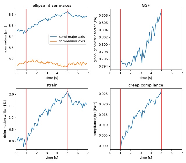
Creep compliance analysis

This example uses the contour data of an HL60 cell in the OS to compute its GGF and creep compliance. The contour data were determined from this phase-contrast video (prior to video compression). During stretching, the total laser power was increased from 0.2W to 1.3W (reflexes due to second harmonic effects appear as white spots).

creep_compliance.py

import ggf
import h5py
import lmfit
import matplotlib.pylab as plt
import numpy as np


def ellipse_fit(radius, theta):
    '''Fit a centered ellipse to data in polar coordinates

    Parameters
    ----------
    radius: 1d ndarray
        radial coordinates
    theta: 1d ndarray
        angular coordinates [rad]

    Returns
    -------
    a, b: floats
        semi-axes of the ellipse; `a` is aligned with theta=0.
    '''
    def residuals(params, radius, theta):
        a = params["a"].value
        b = params["b"].value
        r = a*b / np.sqrt(a**2 * np.sin(theta)**2 + b**2 * np.cos(theta)**2)
        return r - radius

    parms = lmfit.Parameters()
    parms.add(name="a", value=radius.mean())
    parms.add(name="b", value=radius.mean())

    res = lmfit.minimize(residuals, parms, args=(radius, theta))

    return res.params["a"].value, res.params["b"].value


# load the contour data (stored in polar coordinates)
with h5py.File("data/creep_compliance_data.h5", "r") as h5:
    radius = h5["radius"][:] * 1e-6  # [µm] to [m]
    theta = h5["theta"][:]
    time = h5["time"][:]
    meta = dict(h5.attrs)


factors = np.zeros(len(radius), dtype=float)
semimaj = np.zeros(len(radius), dtype=float)
semimin = np.zeros(len(radius), dtype=float)
strains = np.zeros(len(radius), dtype=float)
complnc = np.zeros(len(radius), dtype=float)

for ii in range(len(radius)):
    # determine semi-major and semi-minor axes
    smaj, smin = ellipse_fit(radius[ii], theta[ii])
    semimaj[ii] = smaj
    semimin[ii] = smin
    # compute GGF
    if (time[ii] > meta["time_stretch_begin [s]"]
            and time[ii] < meta["time_stretch_end [s]"]):
        power_per_fiber = meta["power_per_fiber_stretch [W]"]
        f = ggf.get_ggf(
            model="boyde2009",
            semi_major=smaj,
            semi_minor=smin,
            object_index=meta["object_index"],
            medium_index=meta["medium_index"],
            effective_fiber_distance=meta["effective_fiber_distance [m]"],
            mode_field_diameter=meta["mode_field_diameter [m]"],
            power_per_fiber=power_per_fiber,
            wavelength=meta["wavelength [m]"],
            poisson_ratio=.5)
    else:
        power_per_fiber = meta["power_per_fiber_trap [W]"]
        f = np.nan
    factors[ii] = f

# compute compliance
strains = (semimaj-semimaj[0]) / semimaj[0]
complnc = strains / factors
compl_ival = (time > meta["time_stretch_begin [s]"]) * \
    (time < meta["time_stretch_end [s]"])
stretch_index = np.where(compl_ival)[0][0]
complnc_1 = strains/factors[stretch_index]

# plots
plt.figure(figsize=(8, 7))

ax1 = plt.subplot(221, title="ellipse fit semi-axes")
ax1.plot(time, semimaj*1e6, label="semi-major axis")
ax1.plot(time, semimin*1e6, label="semi-minor axis")
ax1.legend()
ax1.set_xlabel("time [s]")
ax1.set_ylabel("axis radius [µm]")

ax2 = plt.subplot(222, title="GGF")
ax2.plot(time, factors)
ax2.set_xlabel("time [s]")
ax2.set_ylabel("global geometric factor [Pa]")

ax3 = plt.subplot(223, title="strain")
ax3.plot(time, (strains)*100)
ax3.set_xlabel("time [s]")
ax3.set_ylabel("deformation $w(t)/r_0$ [%]")

ax4 = plt.subplot(224, title="creep compliance")
ax4.plot(time[compl_ival], complnc[compl_ival])
ax4.set_xlabel("time [s]")
ax4.set_ylabel("compliance $J(t)$ [Pa⁻¹]")

for ax in [ax1, ax2, ax3, ax4]:
    ax.set_xlim(0, np.round(time.max()))
    ax.axvline(x=meta["time_stretch_begin [s]"], c="r")
    ax.axvline(x=meta["time_stretch_end [s]"], c="r")

plt.tight_layout()
plt.show()

Reproduction tests

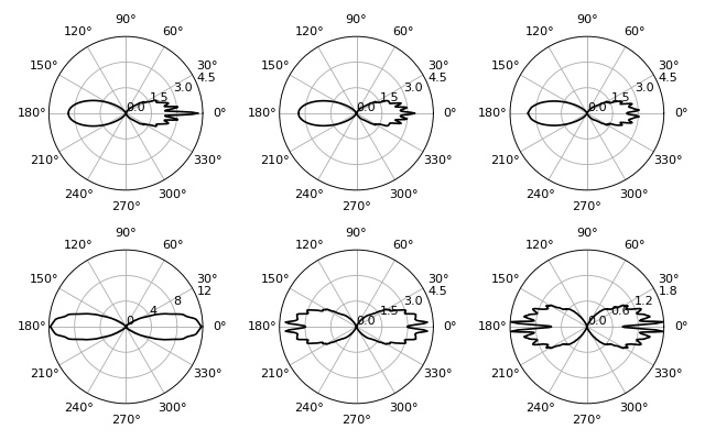
Radial stresses of a prolate spheroid

This examples computes radial stress profiles for spheroidal objects in the optical stretcher, reproducing figures (9) and (10) of [Boyde2009].

stress_reproduced.py

import matplotlib.pylab as plt
import numpy as np
import percache

from ggf.stress.boyde2009.core import stress


@percache.Cache("stress_reproduced.cache", livesync=True)
def compute(**kwargs):
    "Locally cached version of ggf.core.stress"
    return stress(**kwargs)


# variables from the publication
alpha = 47
wavelength = 1064e-9
radius = alpha * wavelength / (2 * np.pi)

kwargs = {"stretch_ratio": .1,
          "object_index": 1.375,
          "medium_index": 1.335,
          "wavelength": wavelength,
          "beam_waist": 3,
          "semi_minor": radius,
          "power_left": 1,
          "power_right": 1,
          "poisson_ratio": 0,
          "n_points": 200,
          }

kwargs1 = kwargs.copy()
kwargs1["power_right"] = 0
kwargs1["stretch_ratio"] = 0
kwargs1["dist"] = 90e-6

kwargs2 = kwargs.copy()
kwargs2["power_right"] = 0
kwargs2["stretch_ratio"] = .05
kwargs2["dist"] = 90e-6

kwargs3 = kwargs.copy()
kwargs3["power_right"] = 0
kwargs3["stretch_ratio"] = .1
kwargs3["dist"] = 90e-6

kwargs4 = kwargs.copy()
kwargs4["dist"] = 60e-6

kwargs5 = kwargs.copy()
kwargs5["dist"] = 120e-6

kwargs6 = kwargs.copy()
kwargs6["dist"] = 200e-6


# polar plots
plt.figure(figsize=(8, 5))

th1, sigma1 = compute(**kwargs1)
ax1 = plt.subplot(231, projection='polar')
ax1.plot(th1, sigma1, "k")
ax1.plot(th1 + np.pi, sigma1[::-1], "k")

th2, sigma2 = compute(**kwargs2)
ax2 = plt.subplot(232, projection='polar')
ax2.plot(th2, sigma2, "k")
ax2.plot(th2 + np.pi, sigma2[::-1], "k")

th3, sigma3 = compute(**kwargs3)
ax3 = plt.subplot(233, projection='polar')
ax3.plot(th3, sigma3, "k")
ax3.plot(th3 + np.pi, sigma3[::-1], "k")

for ax in [ax1, ax2, ax3]:
    ax.set_rticks([0, 1.5, 3, 4.5])
    ax.set_rlim(0, 4.5)

th4, sigma4 = compute(**kwargs4)
ax4 = plt.subplot(234, projection='polar')
ax4.plot(th4, sigma4, "k")
ax4.plot(th4 + np.pi, sigma4[::-1], "k")
ax4.set_rticks([0, 4, 8, 12])
ax4.set_rlim(0, 12)

th5, sigma5 = compute(**kwargs5)
ax5 = plt.subplot(235, projection='polar')
ax5.plot(th5, sigma5, "k")
ax5.plot(th5 + np.pi, sigma5[::-1], "k")
ax5.set_rticks([0, 1.5, 3, 4.5])
ax5.set_rlim(0, 4.5)

th6, sigma6 = compute(**kwargs6)
ax6 = plt.subplot(236, projection='polar')
ax6.plot(th6, sigma6, "k")
ax6.plot(th6 + np.pi, sigma6[::-1], "k")
ax6.set_rticks([0, 0.6, 1.2, 1.8])
ax6.set_rlim(0, 1.8)

for ax in [ax1, ax2, ax3, ax4, ax5, ax6]:
    ax.set_thetagrids(np.linspace(0, 360, 12, endpoint=False))

plt.tight_layout()
plt.show()

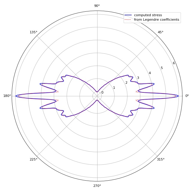
Decomposition of stress in Legendre polynomials

To compute the GGF, ggf.globgeomfact.coeff2ggf() uses the coefficients of the decomposition of the stress into Legendre polynomials \(P_n(\text{cos}(\theta))\). This example visualizes the small differences between the original stress and the stress computed from the Legendre coefficients. This plot is automatically produced by the original Matlab script StretcherNStress.m.

Note that the original Matlab yields different results for the same set of parameters, because the Poisson’s ratio (keyword argument poisson_ratio) is non-zero; see issue #1.

stress_decomposition.py

import matplotlib.pylab as plt
import numpy as np
import percache

from ggf.sci_funcs import legendrePlm
from ggf.stress.boyde2009.core import stress


@percache.Cache("stress_decomposition.cache", livesync=True)
def compute(**kwargs):
    "Locally cached version of ggf.core.stress"
    return stress(**kwargs)


# compute default stress
theta, sigmarr, coeff = compute(ret_legendre_decomp=True,
                                n_points=300)

# compute stress from coefficients
numpoints = theta.size
sigmarr_c = np.zeros((numpoints, 1), dtype=float)
for ii in range(numpoints):
    for jj, cc in enumerate(coeff):
        sigmarr_c[ii] += coeff[jj] * \
            np.real_if_close(legendrePlm(0, jj, np.cos(theta[ii])))

# polar plot
plt.figure(figsize=(8, 8))
ax = plt.subplot(111, projection="polar")
plt.plot(theta, sigmarr, '-b', label="computed stress")
plt.plot(theta + np.pi, sigmarr[::-1], '-b')
plt.plot(theta, sigmarr_c, ':r', label="from Legendre coefficients")
plt.plot(theta + np.pi, sigmarr_c[::-1], ':r')
plt.legend()

plt.tight_layout()
plt.show()

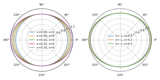
Object boundary: stretching and Poisson’s ratio

This example illustrates how the parameters Poisson’s ratio \(\nu\) and stretch ratio \(\epsilon\) influence the object boundary used in ggf.core.stress() and defined in ggf.core.boundary().

Note that the boundary function was not defined correctly prior to version 0.3.0 (issue #1). Since version 0.3.0, the semi-minor axis is equivalent to the keyword argument a (1 by default).

boundary.py

import numpy as np
import matplotlib.pylab as plt

from ggf.stress.boyde2009.core import boundary

theta = np.linspace(0, 2*np.pi, 300)
costheta = np.cos(theta)

# change epsilon
eps = [.0, .05, .10, .15, .20]
b1s = []
for ep in eps:
    b1s.append(boundary(costheta=costheta,
                        epsilon=ep,
                        nu=.0))

# change Poisson's ratio
nus = [.0, .25, .5]
b2s = []
for nu in nus:
    b2s.append(boundary(costheta=costheta,
                        epsilon=.1,
                        nu=nu))

# plot
plt.figure(figsize=(8, 4))

ax1 = plt.subplot(121, projection="polar")
for ep, bi in zip(eps, b1s):
    ax1.plot(theta, bi, label="ϵ={:.2f}, ν=0".format(ep))
ax1.legend()

ax2 = plt.subplot(122, projection="polar")
for nu, bi in zip(nus, b2s):
    ax2.plot(theta, bi, label="ϵ=.1, ν={:.1f}".format(nu))
ax2.legend()

plt.tight_layout()
plt.show()